A very brief introduction to the skew-normal distribution

This is a very short introduction to the Skew-Normal (SN) distribution. For references to the proper publications, available software and more information, see the SN home-page at http://www.azzalini.it/SN

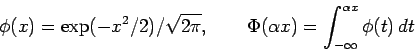
Consider first a continuous random variable $X$ having probability density function of the following form

$$f(x) = 2 \phi(x) \Phi(\alpha x)$$ (1)

where $\alpha$ is a fixed arbitrary number (more about it later), and

$$\phi(x)= \exp(-x^2/2)/\sqrt{2\pi} , \qquad \Phi(\alpha x) = \int_{-\infty}^{\alpha x}\phi(t) dt$$ (2)

denote the standard Normal (Gaussian) density function and its distribution function (the latter evalutated at point $\alpha x$), respectively. The component $\alpha$ is called the shape parameter because it regulates the shape of the density function, as illustrated by some graphs having , and .

The density $f(x)$ enjoys various interesting formal properties. It is easy to check that

1. when $\alpha=0$, the skewness vanishes, and we obtain the standard Normal density,
2. as $\alpha$ increases (in absolute value), the skewness of the distribution increases,
3. when $\alpha\to\infty$, the density converges to the so-called half-normal (or folded normal) density function;
4. if the sign of $\alpha$ changes, the density is reflected on the opposite side of the vertical axis.

The above random variable $X$ and its density function $f(x)$ are the basic components of the construct, but for practical numerical work we need to add location and scale parameters. Consider then the linear transform

$$Y \: =\: \xi + \omega X$$ (3)

which is then said to have a skew-normal distribution with parameters $(\xi, \omega, \alpha),$ and write

$$Y\: \sim\: SN(\xi, \omega^2, \alpha).$$ (4)

We refer to $\xi$, $\omega$ and $\alpha$ as the location, the scale and the shape parameters, respectively. Notice that, when $\alpha=0$, we re-obtain the $N(\xi, \omega^2)$ distribution. You can see additional plots, varying all three parameters, with a demostration program which produces graphs of the univariate skew-normal densities.

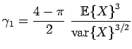
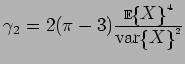
Some characteristic values of the random variable $Y$ are as follows:

	mean value	$\E{Y}= \xi+\omega\:\sqrt{2/\pi} \delta$
	variance	$\var{Y}= \omega^2\;(1-2 \delta^2/\pi)$
	skewness	$\gamma_1 = \dfrac{4-\pi}{2} \; \frac{\E{X}^3}{\var{X}^{3/2}}$
	kurtosis	$\gamma_2 = 2(\pi-3) \frac{\E{X}^4}{\var{X}^{2}}$

where $\delta=\alpha/\sqrt{1+\alpha^2}, \: \E{X}= \sqrt{2/\pi} \delta, \: \var{X}= 1-2 \delta^2/\pi$.

On the statistical side, the skew-normal distribution is often useful to fit observed data with "normal-like" shape of the empirical distribution but with lack of symmetry. You can try it out directly with your data using a form available here.

Ok, but why is it called skew-normal? One reason is implicit in the above passage: this family of distributions includes the standard N(0,1) distribution as a special case, but in general its memebers have a skewed density. Another appealing connection is the fact that

$$X^2 \sim \chi^2_1$$ (5)

irrespective of the value of $\alpha$.

So far for the univariate distribution; a multivariate version also exists. This refers to a multivariate variable $X$ such that

• all its marginal components have a skew-normal distribution;
• its shape is regulated by a vector parameter $\alpha$; when this is 0, we are back to the familiar multivariate normal distribution;
• various other typical properties of the multivariate normal distribution are preserved, in particular: (i) linear transformations of the form $AX$ for any matrix $A$ are still multivariate skew-normal variates, and (ii) the $\chi^2$ distribution of certain quadratic forms is preserved.

A demostration program which produces graphs of the bivariate skew-normal density allows to examine its shape for any given choice of the shape and association parameters.

The present account of the skew-normal distribution is clearly extremely limited. For an extended treatment, see the proper publications.

Back to the Skew-normal distribution